[Hands-On] Building a Real LLM From Scratch for Systems People

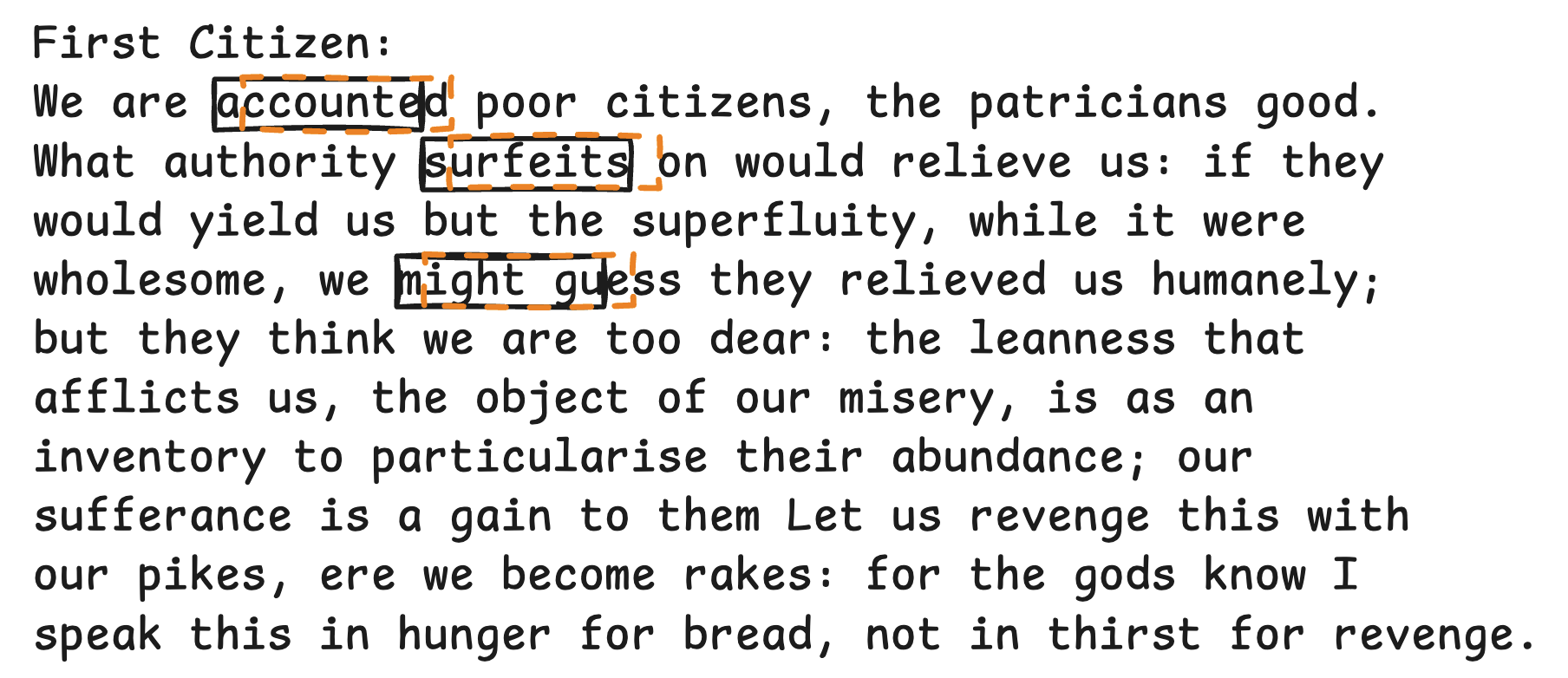
Table of contents

• 1. Introduction
• 2. What will we do in this article?
• 3. What will our LLM do?
• 4. How to train a simple non-language model in PyTorch?
  • What is a tensor? What is an embedding?
  • How to determine the similarity between two embeddings?
  • What is a neural network?
• 5. Making the LLM
  • What do LLMs do?
  • What are tokens?
  • What’s the input and output for the training? What is the training data?
  • Batching
  • We need both semantics and position to understand a token
  • Define embedding tables for semantic and position
  • Convert token IDs and positions to embeddings
  • Merge token meanings and position info
  • Understanding the context
  • What is self-attention?
  • Implement self-attention
  • What’s the output of the model?
  • Calculate the Loss
  • How to generate new text?
• Summary

1. Introduction

By now, we’re probably all familiar with large language models (LLMs) such as ChatGPT, Gemini, and Claude. Since 2022, LLMs have begun to revolutionize the world and have had a significant impact on our lives.

We have been told that LLMs are trained on enormous datasets and generate text by predicting the next token. But this understanding seems superficial. How does it work exactly? As Richard Feynman noted, knowing the name of something is not the same as knowing something.

Systems people should understand LLM internals. As a systems person, I believe systems people should understand LLM internals well. Systems people have deep knowledge of how the infrastructure works. They know how concurrency works. They know sharding. They know OS page management. But they usually know less about machine learning or LLM internals. For example, I didn’t know what “logits” were while working with someone at DeepMind; such gaps create communication friction in collaborations. Systems people should learn the fundamentals of LLMs for the following reasons:

1. Better identify system opportunities for AI
2. Better identify AI opportunities for systems
3. Better collaborate with AI/ML teams (so we speak the same language)
4. Get a sense of the limitations of LLMs.

The above are the overall goals of this article; we achieve these goals by building an LLM from scratch.

2. What will we do in this article?

You will build and run a real GPT model that is trained on Shakespeare’s books and speaks like Shakespeare. Along the way, you will learn the necessary fundamental ML/AI concepts and tools.

This article is from a systems person, for systems people. It is helpful in this way because systems people understand systems people.

At the end, you will be able to:

• understand, build, and run a real GPT model
• get hands-on experience with LLMs
• understand core concepts from embeddings and neural networks to self-attention

We will use a GPT model written by Andrej Karpathy in this article.

The code for this article is available at https://github.com/junhe/llm-from-scratch. We expect you to clone the repo and follow along with the article.

3. What will our LLM do?

To get you excited, let’s see what LLM you will get at the end of this article. You will get an LLM that will write as if it is Shakespeare.

This LLM can do so because it learned from the text of Shakespeare. It is similar to ChatGPT, which is trained on almost all the text in the world.

The following is the text written by the LLM. As you can see, the output has the style of Shakespeare.

(.venv) (base) junhe@Juns-MacBook-Pro-2 llm-0-to-1 % python gpt_complete.py 

step 0: train loss 4.2221, val loss 4.2306
step 500: train loss 1.7434, val loss 1.8896
step 1000: train loss 1.4037, val loss 1.6222
step 1500: train loss 1.2688, val loss 1.5321
step 2000: train loss 1.1918, val loss 1.5063
step 2500: train loss 1.1316, val loss 1.4906
step 3000: train loss 1.0727, val loss 1.4827
step 3500: train loss 1.0164, val loss 1.5064
step 4000: train loss 0.9637, val loss 1.5192
step 4500: train loss 0.9156, val loss 1.5392
step 4999: train loss 0.8574, val loss 1.5730

O BARATHUMBERLANCE:
But never a word than I scape to King Henry,
Before I a high forehereing traops
And hollow the hath or this ceremal.

KING RICHARD IIUS CHARD II:
Touch'd it yon towards,
But the greatest tedious day what the gates:
'Though Clarence is he sworn were breathed
My clie that searloath to this fap, that thou beheld
And heaven shalt us alt thou furnish,
That marges with strongeth age thy oath fearful fame,
With be busher'd with thy birth-swaining blood and tear
Whisp'd stratal arch-

4. How to train a simple non-language model in PyTorch?

We will use PyTorch to build our Shakespeare LLM. Let’s learn how to use PyTorch first, without getting into details of LLMs.

What is a tensor? What is an embedding?

Let’s start with tensors and embeddings. A tensor is simply multidimensional data: a list is a 1-D tensor, and a matrix is a 2-D tensor. In C++ terms (for systems people):

std::vector<int> is a 1-D tensor.

// Create a 3x3 tensor initialized with 0.0
int rows = 3;
int cols = 3;
std::vector<std::vector<double>> tensor(rows, std::vector<double>(cols, 0.0));

Then what is embedding? An embedding is a 1-D tensor that contains numbers of some meanings. For example, let’s imagine that we want to teach computers the meaning of different animals. We can create a vector with two numbers, the first number represents how domesticated it is (-1=Wild, 1=Pet), the second number represents how big it is (-1=Tiny, 1=Huge). By scoring these two features, we create embeddings for them.

Word	Vector (Embedding)	Why?
Dog	[0.7, 0.2]	Very domesticated, medium size.
Cat	[0.8, -0.4]	Very domesticated, small size.
Lion	[-0.9, 0.7]	Very wild, large size.
Tiger	[-0.8, 0.6]	Very wild, large size.
Mouse	[0.1, -0.9]	Mostly wild, very tiny.

Embeddings quantify the features so computers can understand them.

How to determine the similarity between two embeddings?

One magical property of embeddings is that, by turning the animal features into numbers, computers can now determine how similar two animals are. One way is to use the dot product, which we will use later. Let’s use the dot product to answer the question: is a dog more similar to a cat or a lion?

Dog           Cat
[0.7, 0.2] x [0.8, -0.4] = 0.7*0.8 + 0.2*(-0.4) = 0.48

Dog           Lion
[0.7, 0.2] x [-0.9, 0.7] = 0.7*(-0.9) + 0.2*0.7 = -0.49

0.48 is larger than -0.49, so a dog is more similar to a cat than to a lion.

What is a neural network?

I view a neural network as a computer algorithm inspired by the human brain.

• First, it takes some input, and produces some output.
• Second, it learns from the output and adjusts itself.
• Third, it has a neuron-like data structure.

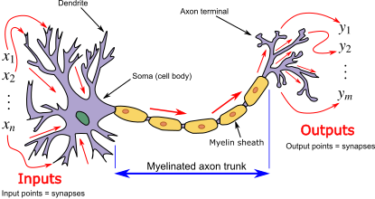
The following is the anatomy of a single artificial neuron.

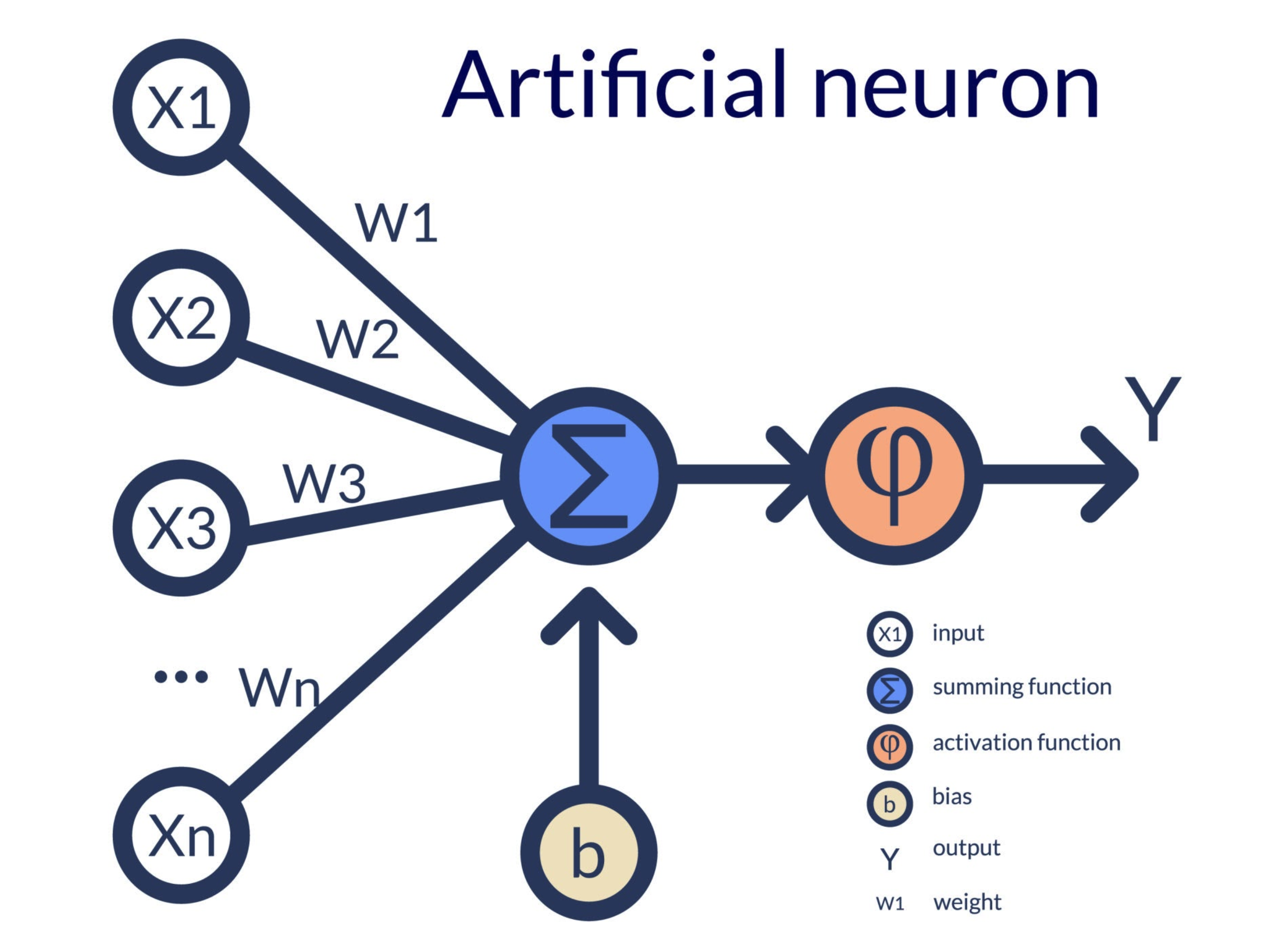
(Anatomy of a single artificial neuron. Source: Тюжина Ирина / Getty Images)

Let’s use a very simple neural network to explain it. Let’s say we want to determine if today is a good day to play outdoor pickleball.

The inputs:

1. Temperature (in Fahrenheit)
2. Wind Speed (in mph)

The weights (the importance)

1. Temperature weight (+0.5): warmer weather generally makes it better for playing
2. Wind speed weight (-2.0): high wind speed ruins the game, so it gets a heavier negative weight.

The bias (the baseline)

Some people like to play more than other people, before any outside factors are considered. Let’s say our bias is 10.

The Summation

Let’s look at a calm, 75°F afternoon in Sunnyvale:

• Temperature contribution: 75°F × 0.5 = 37.5
• Wind contribution: 2 mph × -2.0 = -4.0
• Total Score: 37.5 - 4.0 + 10 (bias) = 43.5

Now let’s look at a cold, blustery day:

• Temperature contribution: 50°F × 0.5 = 25
• Wind contribution: 20 mph × -2.0 = -40
• Total Score: 25 - 40 + 10 (bias) = -5

What are logits?

In this example, the scores 43.5 and -5 are logits, which are raw scores. These raw scores are what computers need, but they are confusing for humans: (1) they have no limits, and (2) they are not probabilities. We usually need to convert the logits to a more unified space so computers and humans can better interpret them.

The Activation Function (The Final Call)

Raw scores of 43.5 and -5 are not very useful predictions. We just want a “yes” or “no”. The activation function is what produces this “yes” or “no” output.

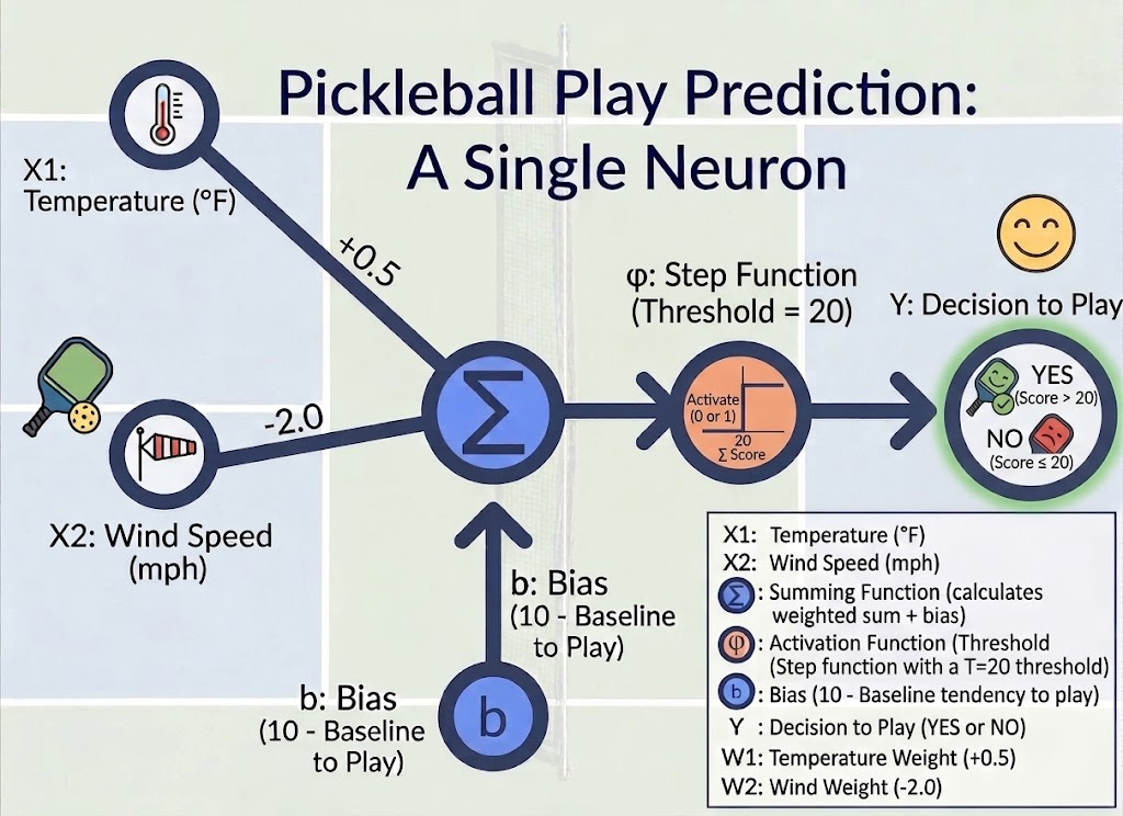
Wait—where do all the weights, bias, and activation come from? In the example above, we manually picked the numbers; but in reality, we don’t know in the beginning. In the beginning of the neural network, these parameters are just random, much like newborn babies have no clue on how wind and temperatures would affect pickleball playing, and babies don’t know how much they like pickleball (i.e., the bias) either. Humans learn by playing. For example, Bob played 5 games and recorded his experience as follows.

Temperature (°F)    Wind Speed (mph)    Play
75.0                3.0                 1.0
80.0                5.0                 1.0
68.0                2.0                 1.0
72.0                15.0                0.0
50.0                20.0                0.0
45.0                8.0                 0.0
85.0                22.0                0.0
65.0                25.0                0.0

Bob learned from the experience above. The next time that he sees temperature 102 and wind 20, he will know that he should not go, because Bob’s brain has been programmed.

The following code is a key part of the training process.

for epoch in range(epochs):
    # Initialize the optimizer, which is an algorithm that will improve the accuracy
    # of the model.
    optimizer.zero_grad()
    
    # Make predictions based on the training input.
    logits = model(X_train)
    # Find out how wrong the predictions are based on the training targets.
    loss = criterion(logits, y_train)
    
    # Note down how to change the parameters based on the loss
    loss.backward()
    # Actually update the parameters.
    optimizer.step()

The following diagram demonstrates one iteration of the process.

1. Feed the model with training inputs
2. Get training outputs (i.e., for the training inputs). The predictions can be very wrong initially.
3. Calculate the loss
4. Use the loss to update the parameters in the model

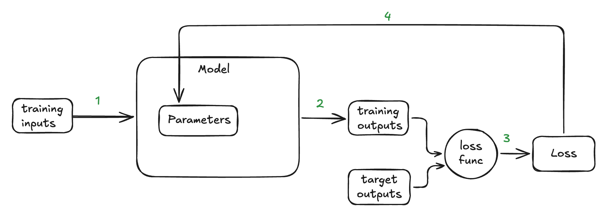
Note that the process above is repeated many times. Each time, the parameters of the model are updated a little bit. The reason we can’t find the right parameters in one shot is that it’s like searching for the bottom of a valley on a foggy hillside. We can’t see anything beyond a few feet around us. So we have to search the hill gradually.

Hands-On (hands_on_001_pickleball.py): Add more training examples to hands_on_001_pickleball.py . Use your common sense to construct 8 examples. Run the program to see if the model makes good predictions.

# ---------------------------------------------------------
# 2. Create Training Data
# ---------------------------------------------------------
# FIXME: Add more training data
# Features: [Temperature (°F), Wind Speed (mph)]
X_raw = torch.tensor([
    [75.0,  3.0],  # Warm, calm -> YES
], dtype=torch.float32)

# Target Labels: 1.0 (YES - Play), 0.0 (NO - Don't Play)
y_train = torch.tensor([
    [1.0],
], dtype=torch.float32)

5. Making the LLM

We have covered the basics of neural networks. Let’s start building the LLM.

What do LLMs do?

LLMs generate text by predicting the next token based on the current text. For example, if the text is “the cat sat on the ___”, the LLM may predict the probability of the possible words like the following:

• “mat” - 72%
• “couch” - 10%
• “floor” - 5%
• “dog” - 2%
• “refrigerator” - 0.001%
• …

If “mat” is selected, then the text for the next round of prediction will become “the cat sat on the mat ___”. This process is repeated to produce long text.

Fundamentally, LLMs predict the next token based on the current context of tokens.

What are tokens?

Humans read text word by word, but that may not be the optimal approach for computers. Tokens are chunks of characters that computers use for processing. There are many ways to tokenize text, which are different ways of splitting words into smaller units. Here are a few examples of tokenizing “Unbelievably, it rained!”

• Word-level: [“Unbelievably”, “,”, “it”, “rained”, “!”]
• Character-level: [“U”, “n”, “b”, “e”, “l”, “i”, “e”, “v”, “a”, “b”, “l”, “y”, …]
• Subword: [“Un”, “believ”, “ably”, “,”, “it”, …]

Modern LLMs use subword tokenization. But we will use character-level tokenization for simplicity in this article.

We also want to convert tokens to token IDs (integers) so that it is easier for computers to work with them. For example, we can put the information of tokens into a matrix, where each row is one token; as a result, we can quickly find information about a token by accessing its row.

In our example, we sort the characters and use the index IDs as token IDs. For example, “hii there” becomes [46, 47, 47, 1, 58, 46, 43, 56, 43].

Hands-On (hands_on_002_tokenization.py): create a decoding lambda.

with open('input.txt', 'r', encoding='utf-8') as f:
    text = f.read()

# here are all the unique characters that occur in this text
chars = sorted(list(set(text)))
vocab_size = len(chars)
# create a mapping from characters to integers
stoi = { ch:i for i,ch in enumerate(chars) }
itos = { i:ch for i,ch in enumerate(chars) }
encode = lambda s: [stoi[c] for c in s] # encoder: take a string, output a list of integers
# FIXME: implement decode function
# decode = 

print(f"chars: {chars}")
print(f"stoi: {stoi}")
print(f"vocab_size: {vocab_size}")
print(f"encode('hii there'): {encode('hii there')}")
# print(f"decode(encode('hii there')): {decode(encode('hii there'))}")
print(''.join(chars))

Answer:

decode = lambda l: ''.join([itos[i] for i in l])

Hands-On (gpt_DIY.py): create the decoding function.

encode = lambda s: [stoi[c] for c in s] # encoder: take a string, output a list of integers
# FIXME-01: implement decode function
decode = ...

Answer:

decode = lambda l: ''.join([itos[i] for i in l])

What’s the input and output for the training? What is the training data?

Recall that, in the earlier pickleball example, we had the following training data. We feed the model X_raw and get some output, then we compare the output with the target output. We see how wrong the model is and then adjust the model.

# Features: [Temperature (°F), Wind Speed (mph)]
X_raw = torch.tensor([
    [75.0,  3.0],  # Warm, calm -> YES
    [80.0,  5.0],  # Warm, light breeze -> YES
    [68.0,  2.0],  # Mild, calm -> YES
    [72.0, 15.0],  # Mild, gusty -> NO
    [50.0, 20.0],  # Cold, windy -> NO
    [45.0,  8.0],  # Cold, light wind -> NO
    [85.0, 22.0],  # Hot, high wind -> NO
    [65.0, 25.0],  # Mild, very windy -> NO
], dtype=torch.float32)

# Target Labels: 1.0 (YES - Play), 0.0 (NO - Don't Play)
y_train = torch.tensor([
    [1.0],
    [1.0],
    [1.0],
    [0.0],
    [0.0],
    [0.0],
    [0.0],
    [0.0]
], dtype=torch.float32)

Now that we want to build a model that can speak like Shakespeare, what will the examples look like? Given the text from Shakespeare, how can we structure the examples to train the model? I think we have all heard that an LLM predicts the next token given the tokens in the context. Let’s take a look at a small example.

The following is a snippet from Shakespeare. We will generate some examples from it for training.

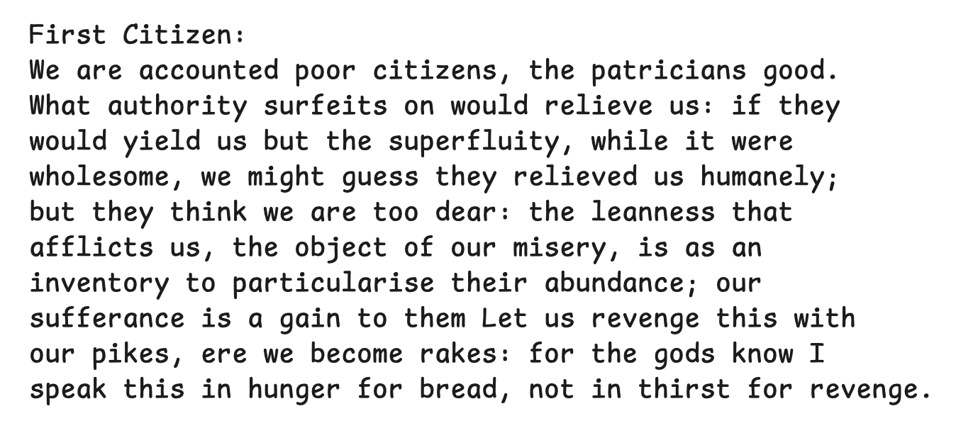
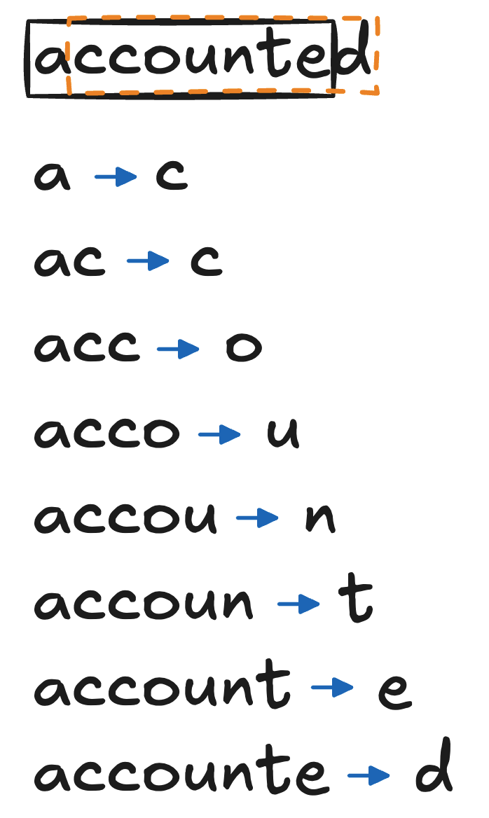
We can use a sliding window of a certain size to create the examples for training, as illustrated below.

We will get the following training examples:

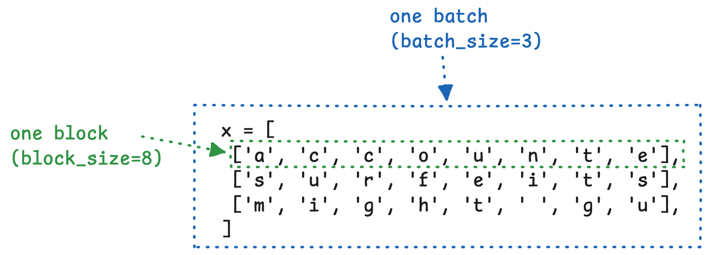
x = [
 ['a', 'c', 'c', 'o', 'u', 'n', 't', 'e'],
 ['s', 'u', 'r', 'f', 'e', 'i', 't', 's'],
 ['m', 'i', 'g', 'h', 't', ' ', 'g', 'u'],
]

y = [
 ['c', 'c', 'o', 'u', 'n', 't', 'e', 'd'],
 ['u', 'r', 'f', 'e', 'i', 't', 's', ' '],
 ['i', 'g', 'h', 't', ' ', 'g', 'u', 'e'],
]

(Note that, in the article we use the actual characters for better illustration. But what actually goes into the model are token IDs, which are integers.)

We actually get 8 examples from the first block.

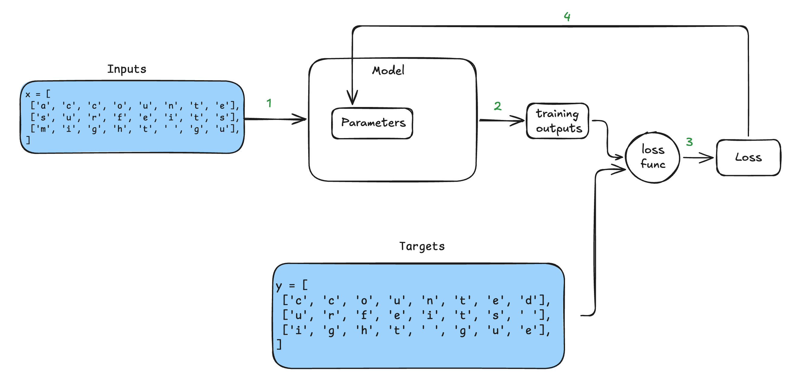
The hope is that, when the model has seen enough examples like these, it will be able to predict the next token. The following diagram shows how the training data is used. The diagram is the same as the pickleball example, except that the temperature and wind speed become a block of text from Shakespeare; the Yes/No becomes the next tokens.

Batching

Earlier we have generated the following training examples.

x = [
 ['a', 'c', 'c', 'o', 'u', 'n', 't', 'e'],
 ['s', 'u', 'r', 'f', 'e', 'i', 't', 's'],
 ['m', 'i', 'g', 'h', 't', ' ', 'g', 'u'],
]

There are 3 rows here. To maximize the efficiency of training (higher parallelism if on GPUs), we want to train on multiple rows at the same time. We call the list of characters (e.g., ['a', 'c', 'c', 'o', 'u', 'n', 't', 'e']) a block. Here the block size is 8, which indicates that there are 8 characters in the list. (In the complete example, the block size is 256.) We call the list of blocks a batch. Here the batch size is 3, which indicates that there are 3 blocks. (In the complete example, the batch size is 64.) The following diagram illustrates the setup.

HandsOn (hands_on_003_training_examples.py): the following code from our LLM is missing the part that fills y.

import torch

text = """First Citizen:
We are accounted poor citizens, the patricians good.
What authority surfeits on would relieve us: if they
would yield us but the superfluity, while it were
wholesome, we might guess they relieved us humanely;
but they think we are too dear: the leanness that
afflicts us, the object of our misery, is as an
inventory to particularise their abundance; our
sufferance is a gain to them Let us revenge this with
our pikes, ere we become rakes: for the gods know I
speak this in hunger for bread, not in thirst for revenge."""

block_size = 8
batch_size = 4

# here are all the unique characters that occur in this text
chars = sorted(list(set(text)))
vocab_size = len(chars)
# create a mapping from characters to integers
stoi = { ch:i for i,ch in enumerate(chars) }
itos = { i:ch for i,ch in enumerate(chars) }
encode = lambda s: [stoi[c] for c in s] # encoder: take a string, output a list of integers
decode = lambda l: ''.join([itos[i] for i in l]) # decoder: take a list of integers, output a string

# Train and test splits
data = torch.tensor(encode(text), dtype=torch.long)

ix = torch.randint(len(data) - block_size, (batch_size,))
print("ix:", ix)
x = torch.stack([data[i:i+block_size] for i in ix])
# FIXME: implement y
y = ...
print('x:\n', x)
print('y:\n', y)
print('decoded x:\n', [decode(x[i].tolist()) for i in range(batch_size)])
print('decoded y:\n', [decode(y[i].tolist()) for i in range(batch_size)])

Quiz (gpt_DIY.py): What is the value of B and T during training?

class GPTLanguageModel(nn.Module):
    ...
    def forward(self, idx, targets=None):
        B, T = idx.shape
        ...

During training, idx is one input batch of token IDs. It is called idx because token IDs are essentially the indexes of tokens in the vocabulary. Here, B is the batch size, which is equal to batch_size , which is 64. T is the block_size, which is 256.

We need both semantics and position to understand a token

(We will use word-level tokenization and an example not from Shakespeare to make it more intuitive to understand.)

Let’s consider the word “bat”: it could mean a piece of baseball gear or a flying animal. The exact meaning can only be determined by the context. The following are two scenarios:

1. Scenario A (Sports): “The top teen player swung the bat.”
2. Scenario B (Nature): “Out of the cave flew a bat.”

Intuitively, to understand a word, the meaning of the word matters and its position in the text also matters. For example, the two sentences above could appear in the same article; the meaning of ‘bat’ depends on its position. So, we need the following parameters to cover semantics and positions.

Token Embedding. For simplicity, let’s assume that the embedding is a vector of size three: [sports score, nature score, emotion score].

Position Embedding. Position also matters. For example, ‘bat’ could appear in an article two times for different meanings. It really depends on where the token is in the document. For example, the embedding could be [document progress, paragraph progress, sentence progress].

Define embedding tables for semantic and position

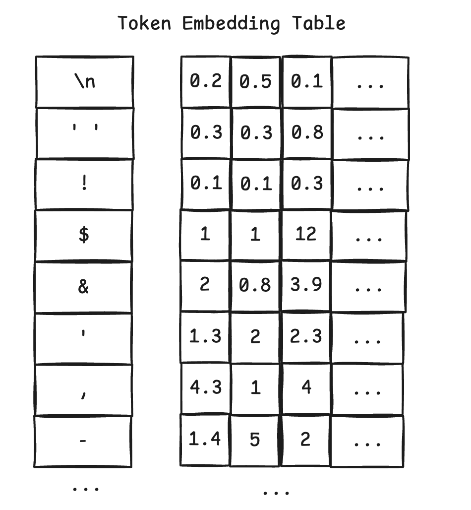
We need a lookup table to contain embeddings for tokens and positions. For the Shakespeare example, the tables can be visualized as follows.

The token embedding has 65 rows, because there are 65 characters in the text. Each row contains the embedding for a token (i.e., a character). For example, the second row has the embedding for ‘!’ (token id is 2).

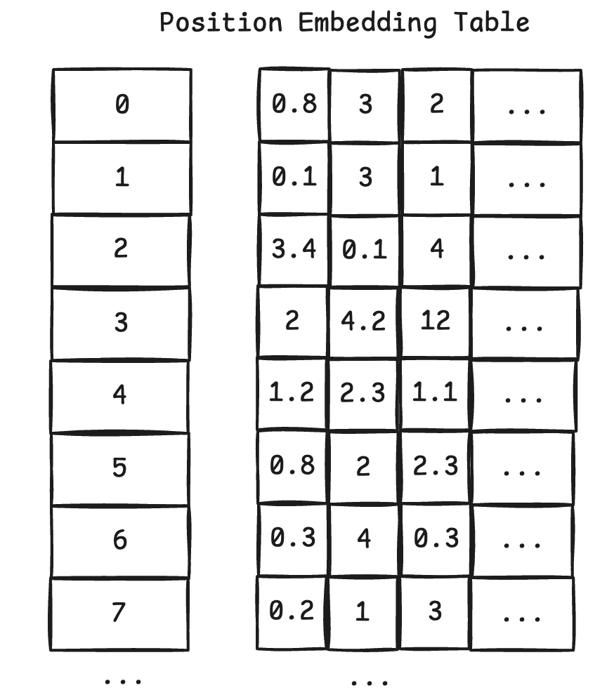
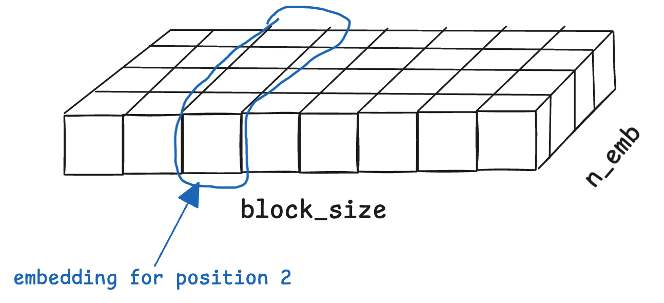
The position embedding table has 256 rows. Each row contains the embedding for a particular position.

In PyTorch, use nn.Embedding to define learnable lookup tables. It is learnable because PyTorch can automatically update the embeddings when optimizing.

HandsOn(hands_on_004_embedding_table.py):

import torch.nn as nn

# Create an embedding table. Each token index maps to a trainable vector.
# FIXME: define the embedding table that stores 5 embeddings, the dimension of
# each embedding is 8.
embedding = nn.Embedding(...)

# Look up the embedding for a single token index
token_id = torch.tensor([2])
single_embedding = embedding(token_id)
print("Single token embedding shape:", single_embedding.shape)
print("Single token embedding:\n", single_embedding)

Answer of HandsOn(hands_on_004_embedding_table.py):

embedding = nn.Embedding(5, 8);

HandsOn (gpt_DIY.py): define the token and position embedding tables.

class GPTLanguageModel(nn.Module):
    def __init__(self):
        super().__init__()
        # each token directly reads off the logits for the next token from a lookup table
        # FIXME-02: define the token embedding table and position embedding table
        self.token_embedding_table = ...
        self.position_embedding_table = ...

        self.blocks = nn.Sequential(*[Block(n_embd, n_head=n_head) for _ in range(n_layer)])
        self.ln_f = nn.LayerNorm(n_embd) # final layer norm
        self.lm_head = nn.Linear(n_embd, vocab_size)

Answer of HandsOn (gpt_DIY.py): FIXME-01:

self.token_embedding_table = nn.Embedding(vocab_size, n_embd)
self.position_embedding_table = nn.Embedding(block_size, n_embd)

Convert token IDs and positions to embeddings

We need to turn the token IDs and their positions into embeddings, which will be optimized during training. Recall that earlier we defined two embedding tables:

self.token_embedding_table = nn.Embedding(vocab_size, n_embd)
self.position_embedding_table = nn.Embedding(block_size, n_embd)

Now we just need to look up the tables. The following code does the lookup for the token meanings.

tok_emb = self.token_embedding_table(idx)

What are the dimensions of tok_emb?

Let’s take the small example we have used. Given the following input

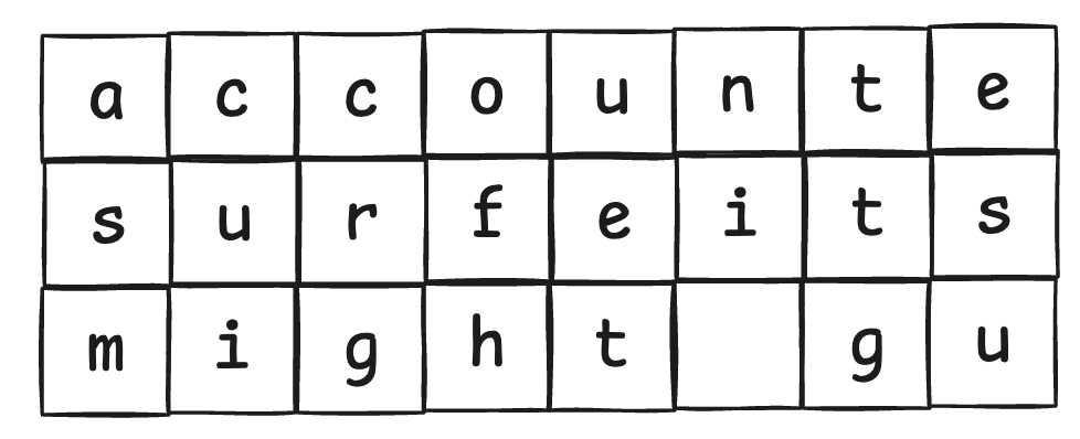
Given the following input, the output will look like the following.

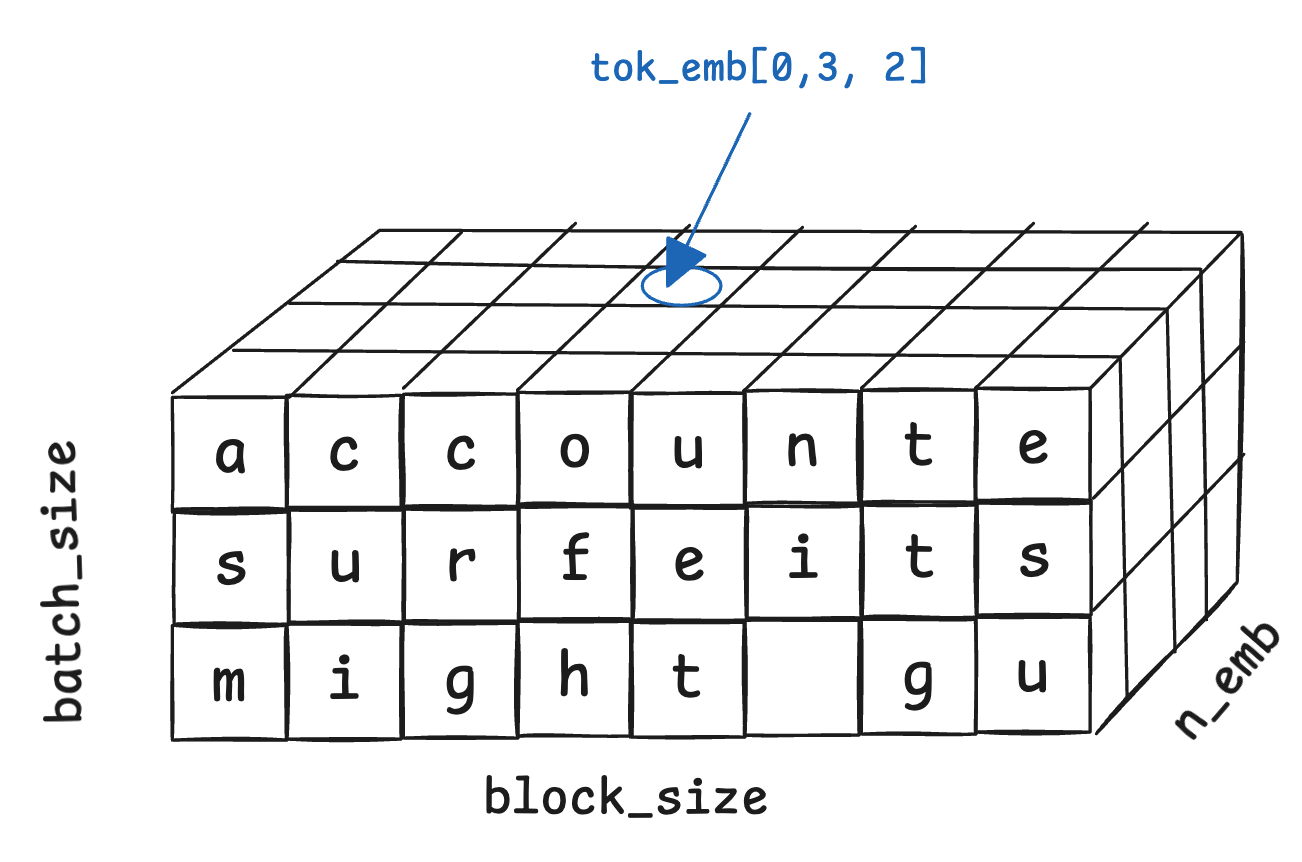
Essentially, for each element in idx, we get an embedding and store it in an additional dimension. For example, tok_emb[0, 3, 2] stores a single number of the embedding for ‘o’. The dimensions of tok_emb are 64x256x384.

Now, let us get the position embeddings. In each block, we have positions 0, 1, …, block_size-1. We just need to look up the position embedding table with this sequence, as follows.

# torch.arange(T) produces [0, 1, 2, ..., T-1]
pos_emb = self.position_embedding_table(torch.arange(T, device=device))

pos_emb can be illustrated as follows.

Merge token meanings and position info

A token can’t be understood without position, so we want to merge them together. We can do this simply by adding the token embedding of a token with its corresponding position embedding. For example, if token embedding is [1, 2, 3] and position embedding is [4, 5, 6], then [1+4, 2+5, 3+6] = [5, 7, 9] is an embedding that contains both meaning and position info.

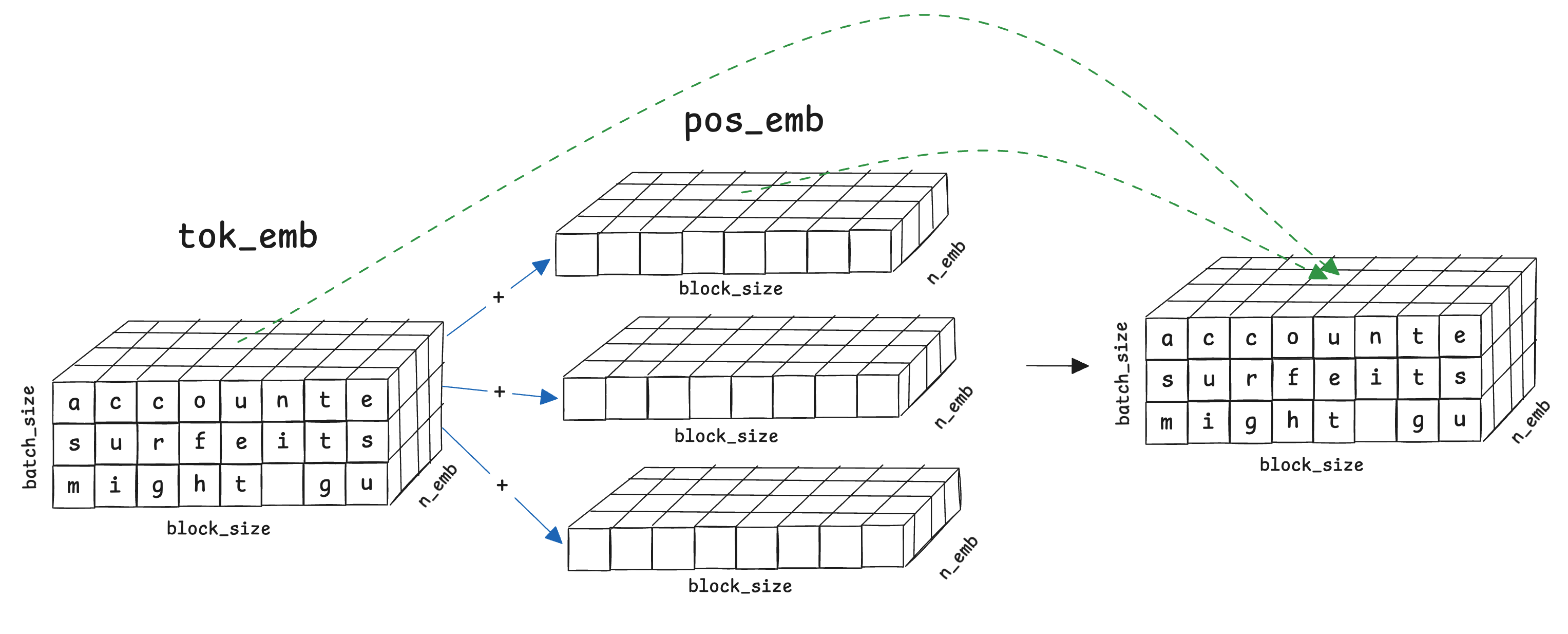
The resulting embedding will then contain values from the token itself and its position.

HandsOn (hands_on_005_merge_token_and_pos.py):

import torch

# 3x8x4 concrete token embeddings
tok_emb = torch.tensor([
    [[1, 2, 3, 4], [5, 6, 7, 8], [9, 10, 11, 12], [13, 14, 15, 16], [17, 18, 19, 20], [21, 22, 23, 24], [25, 26, 27, 28], [29, 30, 31, 32]],
    [[41, 42, 43, 44], [45, 46, 47, 48], [49, 50, 51, 52], [53, 54, 55, 56], [57, 58, 59, 60], [61, 62, 63, 64], [65, 66, 67, 68], [69, 70, 71, 72]],
    [[81, 82, 83, 84], [85, 86, 87, 88], [89, 90, 91, 92], [93, 94, 95, 96], [97, 98, 99, 100], [101, 102, 103, 104], [105, 106, 107, 108], [109, 110, 111, 112]]
], dtype=torch.float32)

# 8x4 concrete position embeddings
pos_emb = torch.tensor([
    [0.1, 0.2, 0.3, 0.4],
    [0.5, 0.6, 0.7, 0.8],
    [0.9, 1.0, 1.1, 1.2],
    [1.3, 1.4, 1.5, 1.6],
    [1.7, 1.8, 1.9, 2.0],
    [2.1, 2.2, 2.3, 2.4],
    [2.5, 2.6, 2.7, 2.8],
    [2.9, 3.0, 3.1, 3.2]
], dtype=torch.float32)

# FIXME:
# Add the two tensors. PyTorch broadcasts pos_emb from (8, 4) to (3, 8, 4).
x = ...

print("tok_emb shape:", tok_emb.shape)
print("pos_emb shape:", pos_emb.shape)
print("x = tok_emb + pos_emb shape:", x.shape)
print(x)
 

Answer of HandsOn (hands_on_005_merge_token_and_pos.py):

x = tok_emb + pos_emb

HandsOn (gpt_DIY.py): merge the tok_emb and pos_emb.

tok_emb = self.token_embedding_table(idx)
pos_emb = self.position_embedding_table(torch.arange(T, device=device))
x = ...

HandsOn (gpt_DIY.py):

x = tok_emb + pos_emb

As a reminder, these embeddings are random initially. The goal is to learn these parameters, just like how we learned the parameters in the pickleball example.

Understanding the context

We have combined the token meaning and position into one tensor, but the tokens are still isolated: the combined embedding only contains the info of one token. We must understand the context, which is the tokens at and before a particular token in a block, in order to really understand a token and predict the next token. The following diagram illustrates the goal; for example, the embedding of ‘o’ should contain the information of ‘a’, ‘c’, ‘c’ and ‘o’, which is the context.

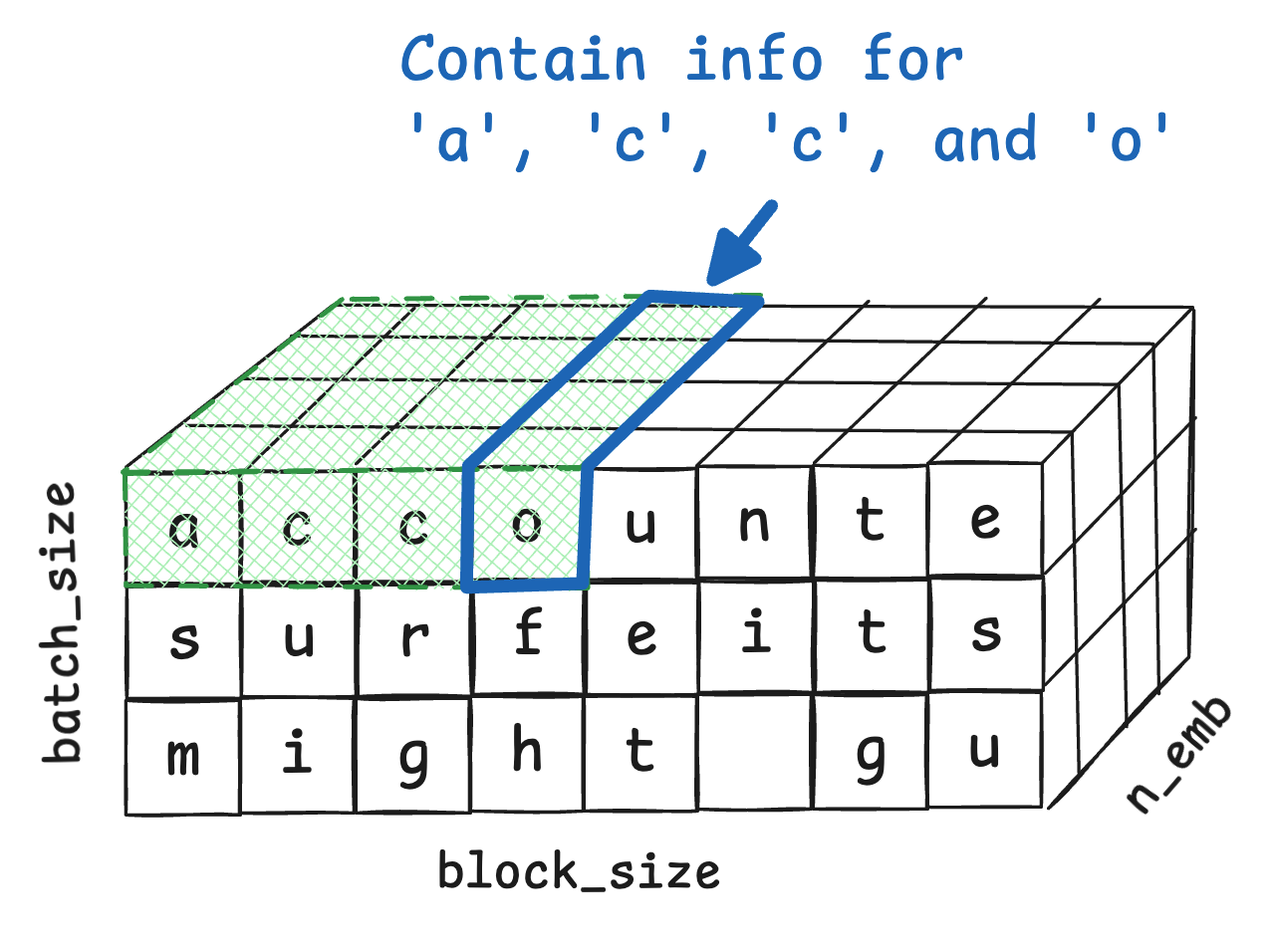
GPT understands the context by a mechanism called self-attention, which is the key part of modern LLMs. Let’s step back and look at a more intuitive example to understand it, then we will come back to the Shakespeare example, which uses the less intuitive character-level tokenization.

What is self-attention?

Let’s look at the ‘bat’ example again.

1. Scenario A (Sports): “The top teen player swung the bat.”
2. Scenario B (Nature): “Out of the cave flew a bat.”

The goal of LLMs is to predict the next token based on the tokens in the context. So, when we try to understand the token in a block (i.e., learn the token embedding and position embedding), we will need to collect information of tokens at and before the particular token. Let’s look at an example.

Let’s say we have some scores for a feature for the different tokens. Now we want to collect scores for understanding ‘bat’. One way is to sum the scores. The result is 0.3+0.5+2+1.3+3+0.3+2.4=9.8.

This approach can collect info, but it also makes the collected score depend on the number of tokens before it. We don’t want this because it will generally make the token that appears later in the context have a larger score. We can solve the problem by averaging the score. It then becomes 9.8/7=1.4. This is better.

But some tokens are clearly more important to ‘bat’ than others; ‘bat’ should pay more attention to them. So, we should add a weight for each token to indicate how much attention it should receive. The new score of bat becomes w_1*0.3+w_2*0.5+w_3*2+w_4*1.3+w_5*3+w_6*0.3+w_7*2.4 .

How can we determine the weight? The self-attention mechanism uses two matrices to do it. They are ‘query’ and ‘key’.

• Q (query): what information should I look for at my position? For example, a query of “bat” at a certain position could have a query “I look for information about sports, nature”. Then the over-simplified Q may be [1, 1, 0] .
• K (key): what quick information does the token provide at its position? For example, the token ‘player’ could be learned and become [0.9, 0.2, 0.1], which indicates that “I am related to sports, not so much about nature or emotion”. The token ‘the’ could have key [0.1, 0.1, 0.1], indicating that it is not so much about sports, nature, or emotion.

For example, let’s get the weights of ‘The’ and ‘player’; in other words, let’s check which of ‘The’ and ‘player’ is more related to ‘bat’. This is done by getting the product of the query of ‘bat’ and the keys of ‘the’ and ‘player’.

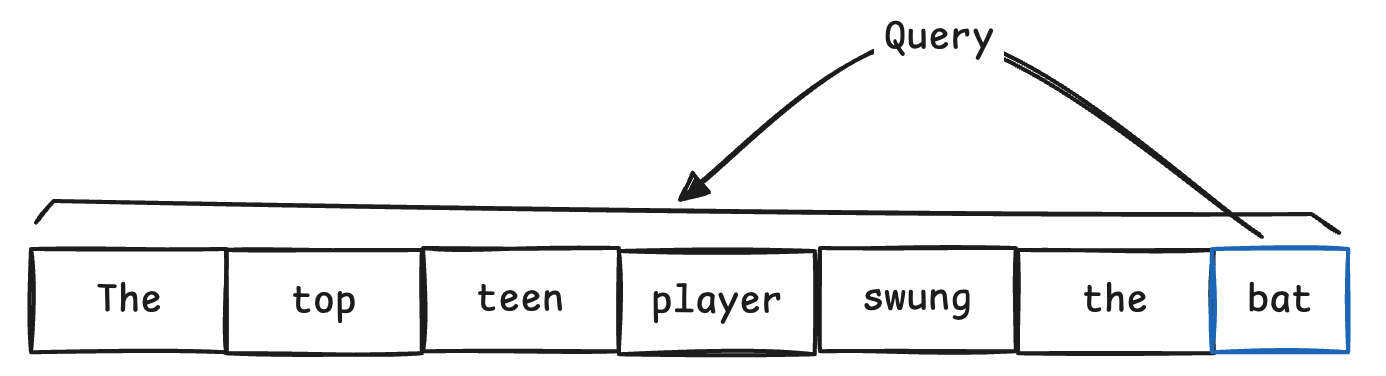
• Query(’bat’) @ Key(’the’) = [1, 1, 0] @ [0.1, 0.1, 0.1] = 1*0.1+1*0.1+0*0.1 = 0.2
• …
• Query('bat') @ Key('player') = [1, 1, 0] @ [0.9, 0.2, 0.1] = 1*0.9+1*0.2+0*0.1 = 1.1
• …

In the end, we may get the following weight.

Q and K are for calculating the weight. We also need V (value):

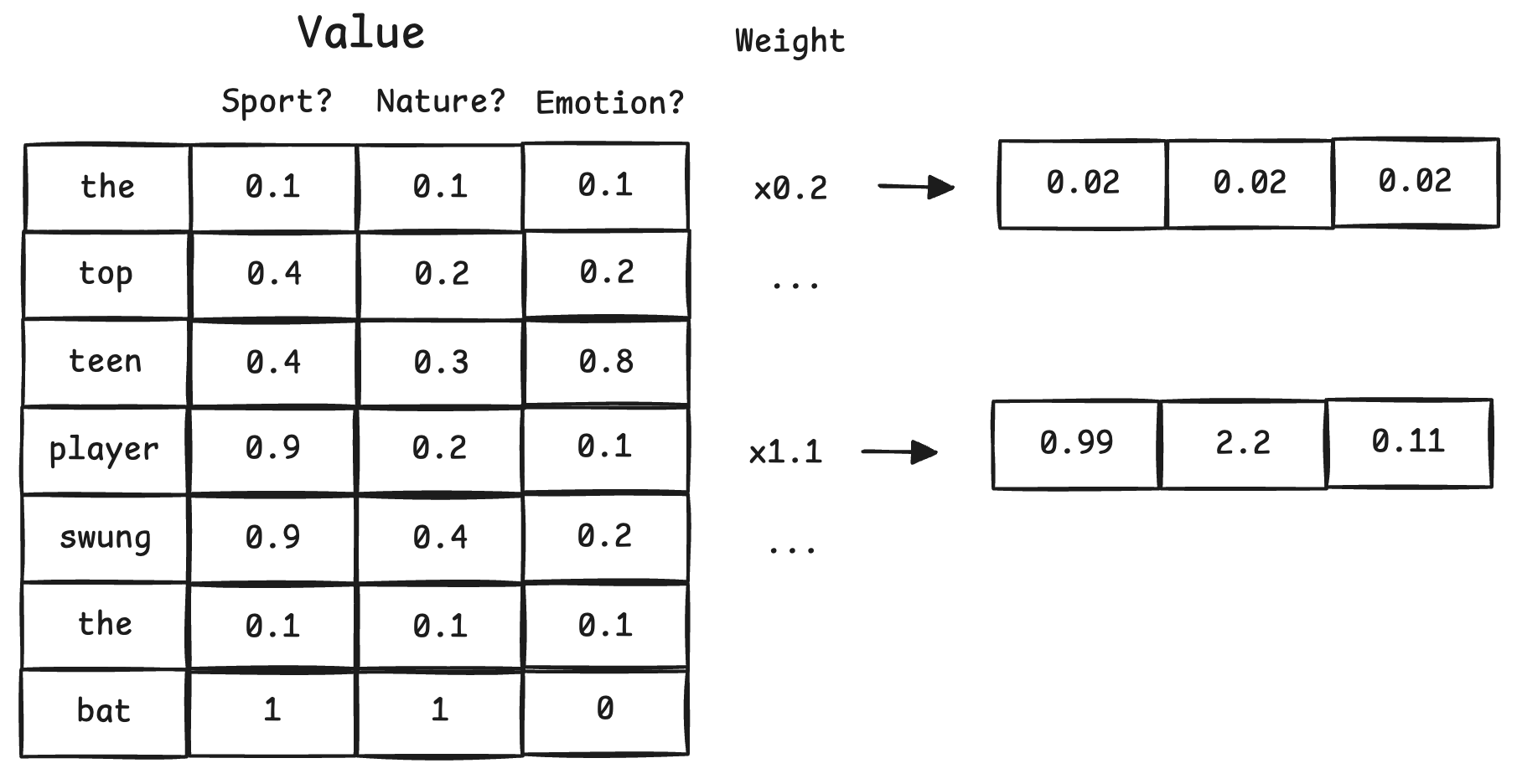
• V (value): what actual meaning does the token provide at its position if someone pays attention to it? For example, the value of the token ‘player’ could be [1, -1, -1] , indicating that the word is sporty, not so much about nature or emotion.

As you can see, ‘player’ relates to ‘bat’ more than ‘the’, because 1.1 > 0.2. So bat will pay more attention to ‘player’ than ‘the’, which is done by scaling the values. For example,

As we can see, the value of ‘player’ becomes more important than ‘the’; in other words, when trying to understand ‘bat’, we will pay more attention to ‘player’ than ‘the’. This makes sense because ‘player’ is about sports, which helps in understanding ‘bat’. In the end, for any position t, we will have block[t] containing information at and before t, as illustrated below.

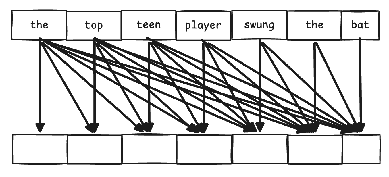
Note that we have used the query of ‘bat’ to match the tokens before and including it, to understand ‘bat’. In fact, we have to do the same for all tokens, to understand all tokens.

Why do we need Query and Key? Query controls what we look for. For example, even if ‘bat’ has meanings about sports and nature in itself, it may not want to look for nature-related tokens, because we have found that this particular ‘bat’ is the baseball bat. Key can control what is exposed to the query. There could be cases where the token has meanings about nature but does not want to let others know about it because the particular token is not about nature.

Why do we need both K and V? V contains the actual meaning, and K controls what parts of V, and how much of them, are exposed, depending on the query. An analogy would be: Q is like a customer at a bookstore, looking for a book; K is like the author. Q and K will talk, then K will bring the book (V) that the customer needs. Or even more accurately, K will actually read the book to Q, skipping information that isn’t relevant to Q, according to Q’s needs.

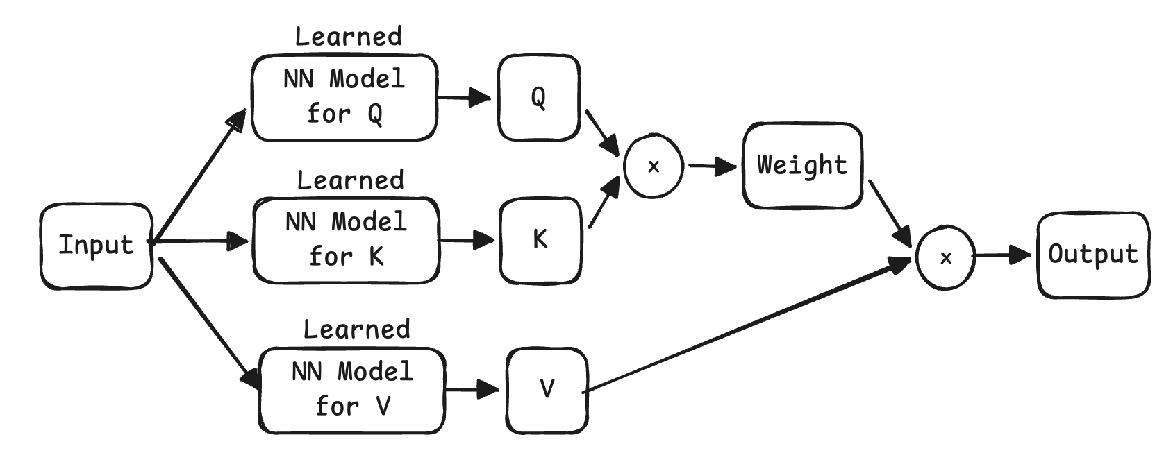
Where do Q, K, and V come from? Note that Q, K, V are matrices produced by their corresponding linear layers. The following is an illustration of how the data flows. The input is a tensor with token meaning and position info. The input is fed into three models: one model learns how to build Query, one model learns how to build K, and one model learns how to build V. Then Q and K are used to determine a weight matrix, which is used to determine what features we extract from V.

HandsOn (gpt_DIY.py): the definition of self.query is missing. Please define it.

class Head(nn.Module):
    """ one head of self-attention """

    def __init__(self, head_size):
        super().__init__()
        self.key = nn.Linear(n_embd, head_size, bias=False)
        # FIXME-03: define the query layer
        self.query = ...
        self.value = nn.Linear(n_embd, head_size, bias=False)

Answer of Hands-On (gpt_DIY.py):

self.query = nn.Linear(n_embd, head_size, bias=False)

Implement self-attention

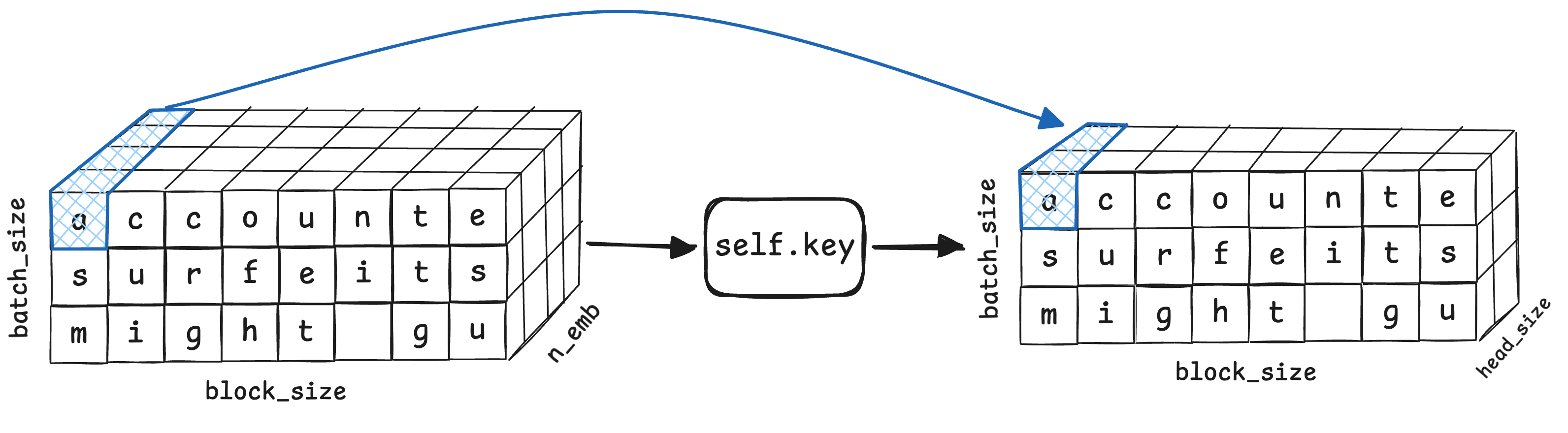
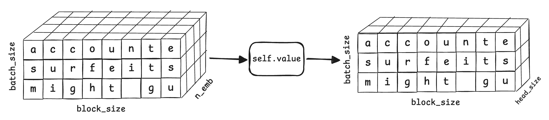
The input to the attention layer is the ‘sum of semantics and position’. If we feed it to self.key, it will become the following (note that the output size of self.key is head_size).

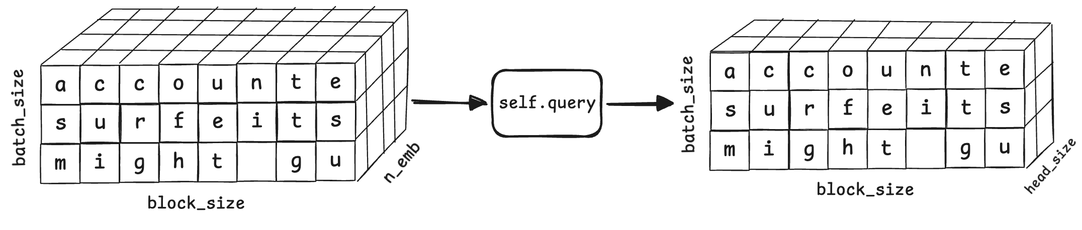
The query can be obtained similarly.

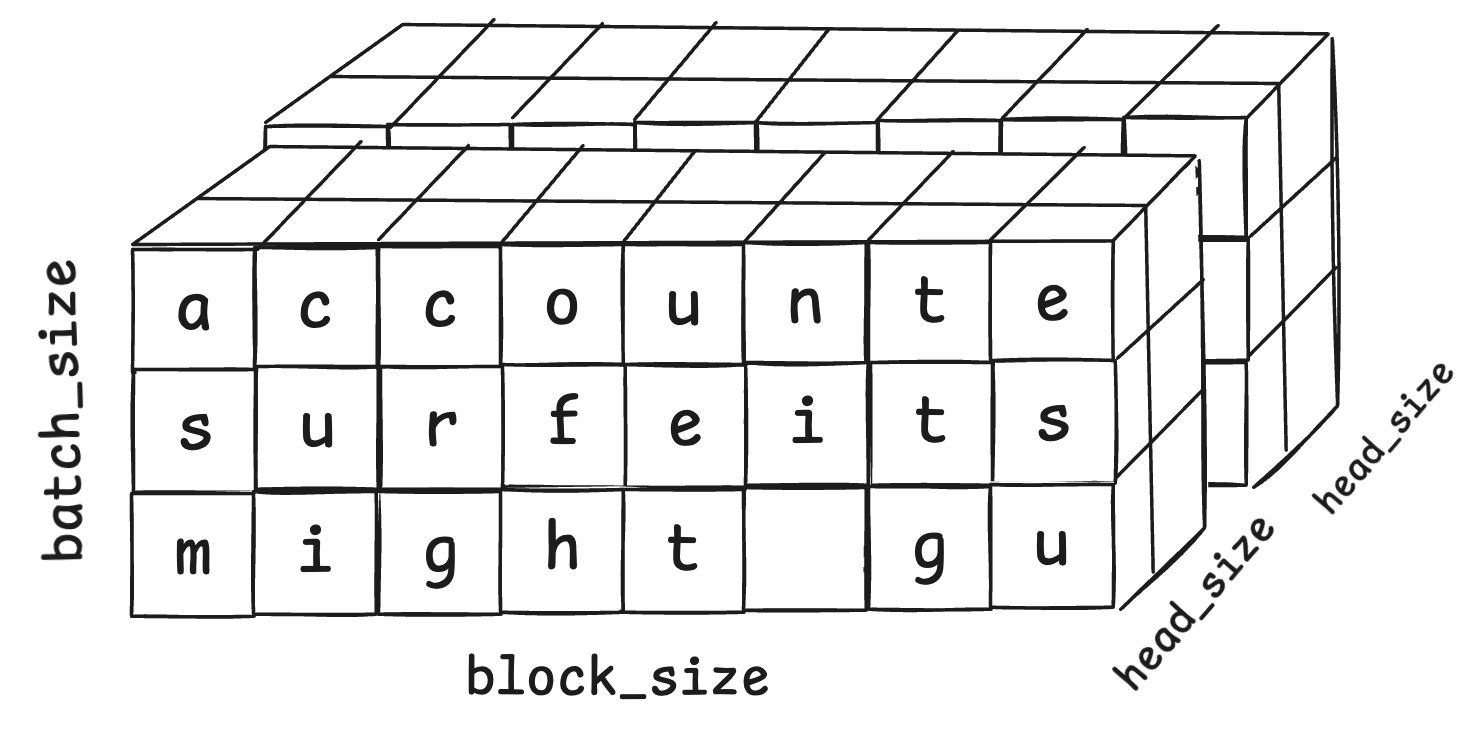
Here is where we should explain what “multi-head attention” is. Multi-head attention is just multiple self-attention pipelines running independently, whose results are then simply concatenated together. Because we need to concatenate the results, each head should only produce an embedding of size n_emb//n_head. The following diagram demonstrates how two results are concatenated.

HandsOn (hands_on_006_multi_head_contatenation.py): concatenate two tensors. The results of multi-head attentions are concatenated in a similar way.

import torch

# Two 3x8x2 attention-head outputs.
# Shape: (batch_size=3, seq_len=8, head_dim=2)
head_1 = torch.tensor([
    [[1, 2], [3, 4], [5, 6], [7, 8], [9, 10], [11, 12], [13, 14], [15, 16]],
    [[17, 18], [19, 20], [21, 22], [23, 24], [25, 26], [27, 28], [29, 30], [31, 32]],
    [[33, 34], [35, 36], [37, 38], [39, 40], [41, 42], [43, 44], [45, 46], [47, 48]]
], dtype=torch.float32)

head_2 = torch.tensor([
    [[0.1, 0.2], [0.3, 0.4], [0.5, 0.6], [0.7, 0.8], [0.9, 1.0], [1.1, 1.2], [1.3, 1.4], [1.5, 1.6]],
    [[1.7, 1.8], [1.9, 2.0], [2.1, 2.2], [2.3, 2.4], [2.5, 2.6], [2.7, 2.8], [2.9, 3.0], [3.1, 3.2]],
    [[3.3, 3.4], [3.5, 3.6], [3.7, 3.8], [3.9, 4.0], [4.1, 4.2], [4.3, 4.4], [4.5, 4.6], [4.7, 4.8]]
], dtype=torch.float32)

# FIXME:
# Concatenate the two heads along the last dimension (head_dim).
# The resulting shape is (3, 8, 4), combining the two head dimensions.
out = ...

print("head_1 shape:", head_1.shape)
print("head_2 shape:", head_2.shape)
print("concatenated output shape:", out.shape)
print(out)

HandsOn (hands_on_006_multi_head_contatenation.py):

out = torch.cat([head_1, head_2], dim=-1)

Now, as we discussed in the ‘bat’ example, we need to get the dot product of query and key. This is done by q @ k.transpose(-2,-1) in PyTorch.

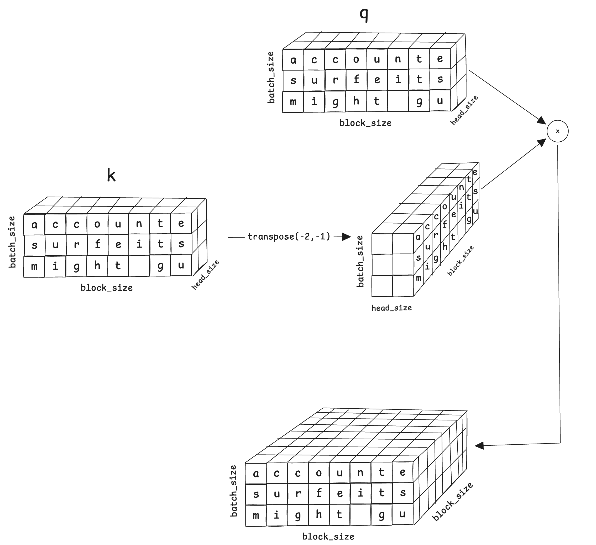
The trick to quickly understand the manipulation is to look at only one block. For example, looking at the row of ‘t’ in weight, it contains how much attention ‘t’ should pay to other tokens in the same block.

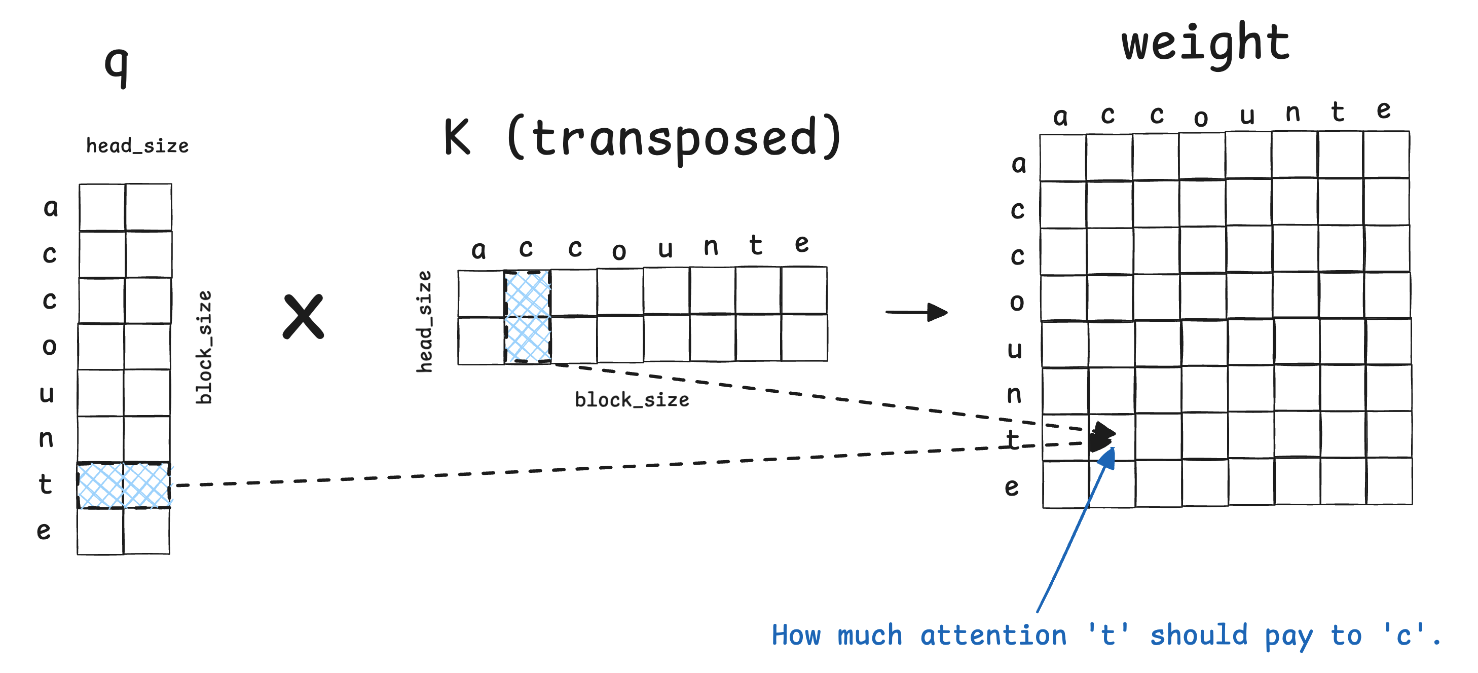
Recall that, for any token, we should only look at the token itself and the tokens before it. But the weight matrix right now contains weights we don’t want. For example, the cell pointed to by an arrow below tells how much ‘t’ should pay attention to ‘e’, which is after ‘t’. It is easy to see that the top-right half of the matrix contains such unwanted values. We don’t want to include them in the results.

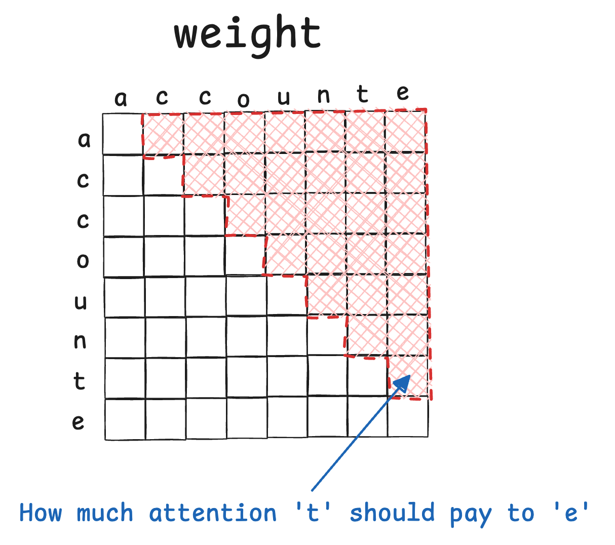
HandsOn (hands_on_007_masking.py): set the red part (upper triangle) to -inf.

import torch
import torch.nn.functional as F

T = 8

self_tril = torch.tril(torch.ones(T, T))
print("self.tril[:T, :T]:")
print(self_tril)
print()

wei = torch.tensor([
    [ 1.0,  2.0,  3.0,  4.0,  5.0,  6.0,  7.0,  8.0],
    [ 9.0, 10.0, 11.0, 12.0, 13.0, 14.0, 15.0, 16.0],
    [17.0, 18.0, 19.0, 20.0, 21.0, 22.0, 23.0, 24.0],
    [25.0, 26.0, 27.0, 28.0, 29.0, 30.0, 31.0, 32.0],
    [33.0, 34.0, 35.0, 36.0, 37.0, 38.0, 39.0, 40.0],
    [41.0, 42.0, 43.0, 44.0, 45.0, 46.0, 47.0, 48.0],
    [49.0, 50.0, 51.0, 52.0, 53.0, 54.0, 55.0, 56.0],
    [57.0, 58.0, 59.0, 60.0, 61.0, 62.0, 63.0, 64.0],
], dtype=torch.float32)
print("wei before masked_fill:")
print(wei)
print()

# FIXME
# Set the upper triangle to -inf.
wei = wei.masked_fill(..., float('-inf'))
print("wei after masked_fill (future positions set to -inf):")
print(wei)
print()

HandsOn (gpt_DIY.py): set the upper triangle to be -inf.

The answer for the two HandsOns above is as follows. We will soon see why we set it to -inf instead of 0.

wei = wei.masked_fill(self.tril[:T, :T] == 0, float('-inf'))

Let’s assume the weight for the ‘t’ row is as follows. We want to turn the numbers into probabilities with sum 1, because we want ‘weighted average’, which keeps the Value at the same scale. In other words, we say “I have one unit of attention to spend, distribute it across the sources”. If the sum is a random number, different rows in the matrix may be scaled differently and not comparable.

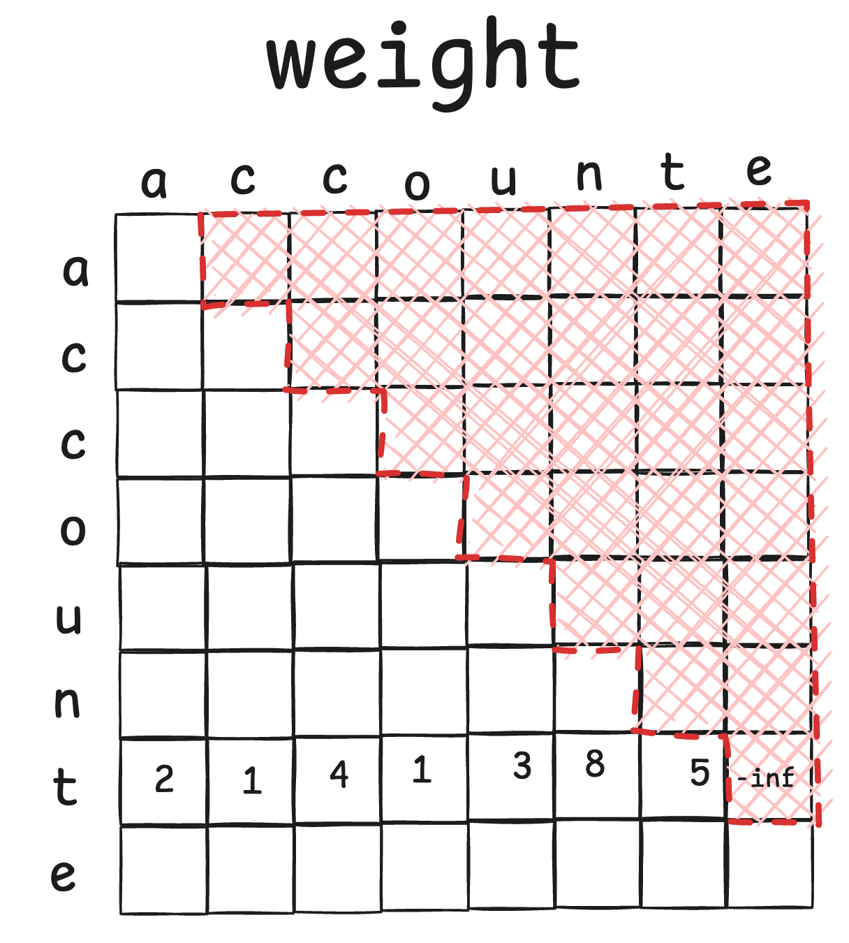
The code uses Softmax to turn the numbers into probabilities.

wei = F.softmax(wei, dim=-1) # do softmax at the last dimension.

Softmax is essentially the following.

\[p_i = \frac{e^{z_i}}{\sum_j e^{z_j}}\]

So the original numbers become

\[\text{Softmax}(2) = \frac{e^2}{e^2 + e^1 + e^4 + e^1 + e^3 + e^8 + e^5 + e^{-\infty}} \approx 0.0023\] \[\text{Softmax}(1) = \frac{e^1}{e^2 + e^1 + e^4 + e^1 + e^3 + e^8 + e^5 + e^{-\infty}} \approx 0.0008\] \[\text{Softmax}(4) = \frac{e^4}{e^2 + e^1 + e^4 + e^1 + e^3 + e^8 + e^5 + e^{-\infty}} \approx 0.0170\] \[\text{Softmax}(1) = \frac{e^1}{e^2 + e^1 + e^4 + e^1 + e^3 + e^8 + e^5 + e^{-\infty}} \approx 0.0008\]

…

\[\text{Softmax}(-\infty) = \frac{e^{-\infty}}{e^2 + e^1 + e^4 + e^1 + e^3 + e^8 + e^5 + e^{-\infty}} = 0.0000\]

The result is as follows.

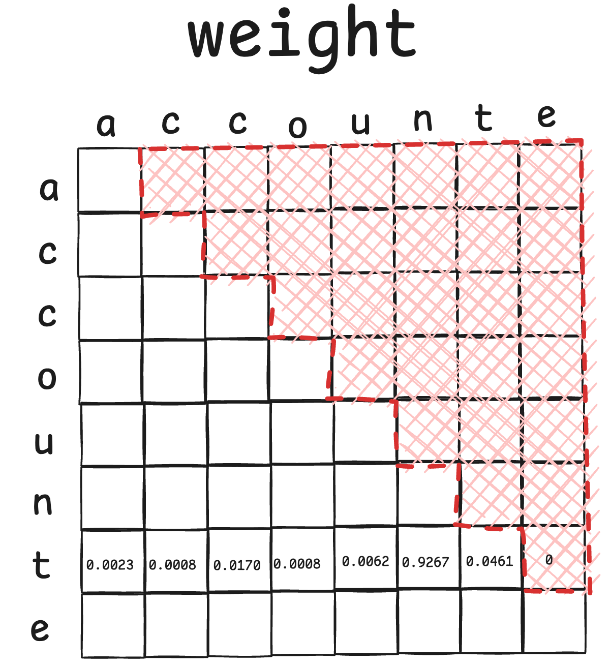
Note that the ‘t-e’ cell becomes 0 because

\[e^{-\infty} = 0\]

HandsOn (hands_on_008_softmax.py): add 3 numbers to weight , with at least one -inf, and then observe the results. What’s the sum? What does -inf become?

import torch
import torch.nn.functional as F

# FIXME
# Add 3 numbers, with at least one -info.
weight = torch.tensor([...])
print("Input:", weight)

probs = F.softmax(weight, dim=0)
print("Softmax probabilities:", probs)
print("Sum of probabilities:", probs.sum().item())

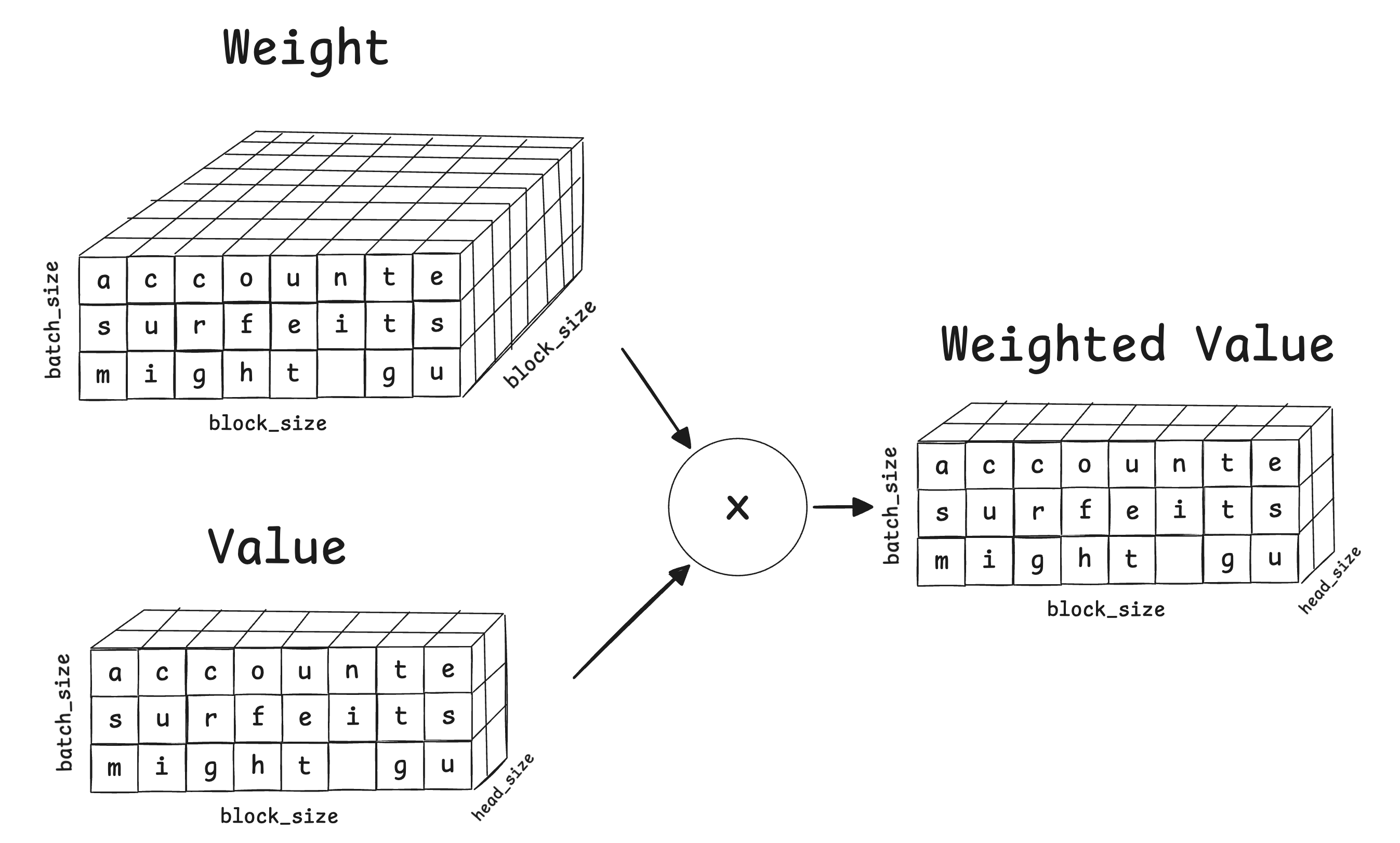
Now we come to the last step: getting the weighted Value. Similar to how we get k and q, we use self.value to get the matrix v. Recall that v is the actual info each token wants to expose.

The following diagram demonstrates the process to get weighted value.

To more intuitively understand it, let’s again look at one single block (i.e., a flat horizontal layer in the diagram above).

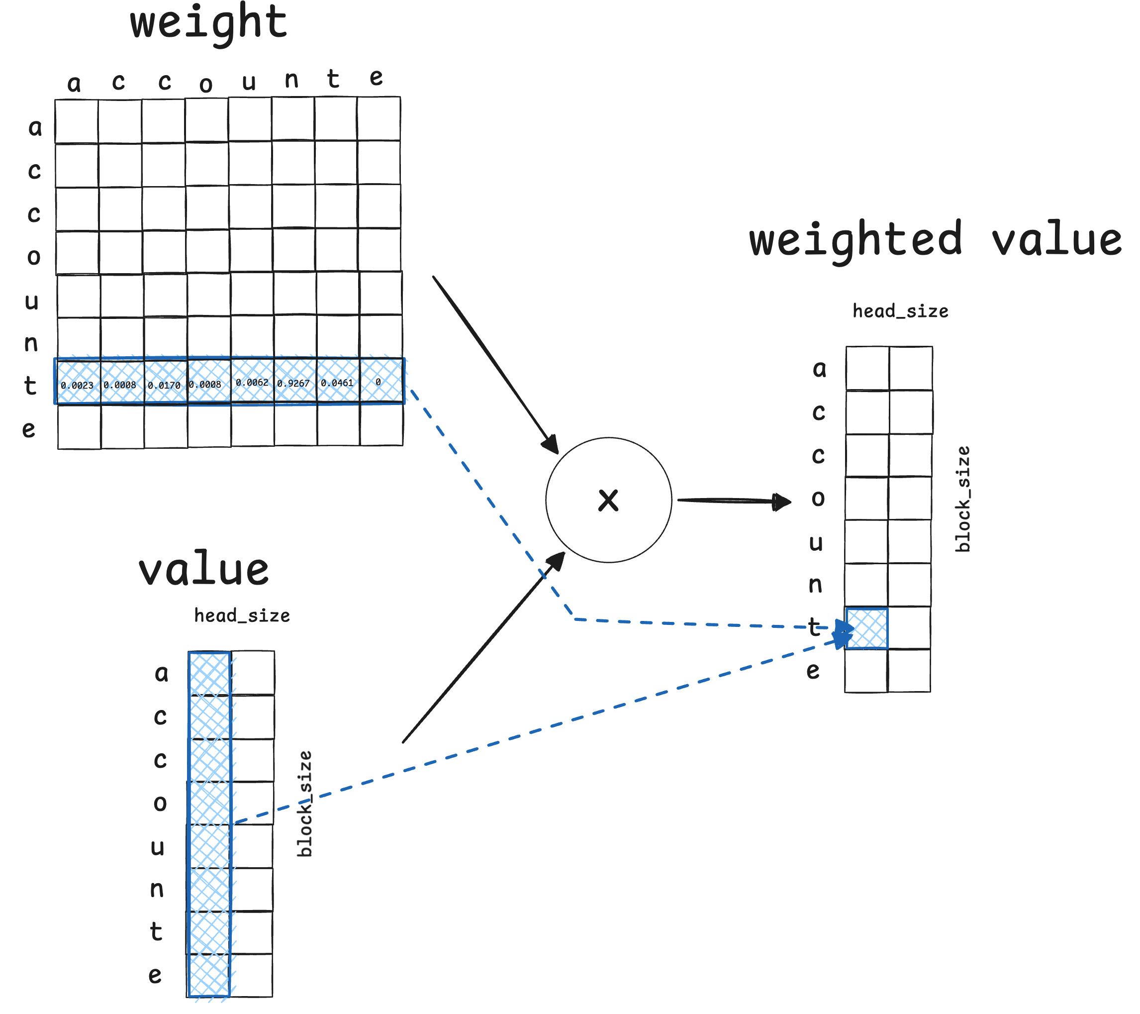
For example, the highlighted cell in the weighted value is the dot product of the weight of the ‘t’ row and the first column of the value. In the end, the highlighted cell in weighted value has aggregated info from all tokens at and before its position.

What’s the output of the model?

So far, we have obtained the weighted value. But that’s not what we want in the end. We want to predict the next token. In other words, we want to know the probabilities of all tokens in the vocabulary for being the next token. For example, given the context ‘accoun’, the probability of ‘t’ being the next may be 0.4 and the probability of ‘&’ may be 0.003.

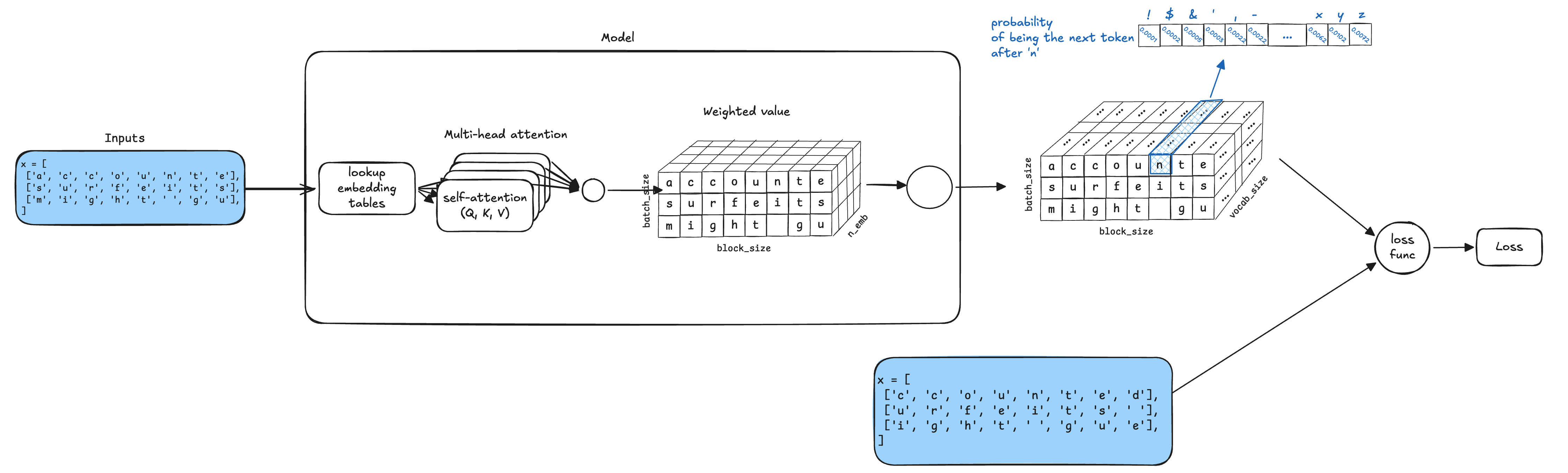
How can we turn the weighted value into probabilities of next tokens? Well, just run the data through a model. The training examples will teach the model to produce the probabilities.

HandsOn (gpt_DIY.py): define the model that turns the weighted value to probabilities of next tokens.

# FIXME-04: define the model that maps the embedding to the vocabulary
# probabilities
self.lm_head = ...

FIXME-04 Answer:

self.lm_head = nn.Linear(n_embd, vocab_size)

Calculate the Loss

The model outputs the probabilities of the next token, and we know the correct next token. How can we calculate how wrong the outputs are (i.e., the loss)? The loss is the following.

\[\text{Loss} = -\log(p_{\text{correct}})\]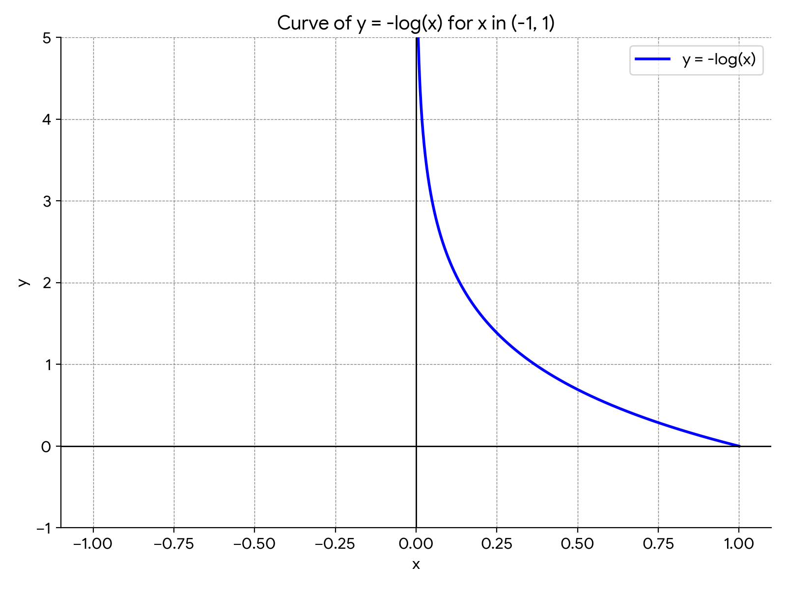

Looking at the plot, you can see that the lower the probability of the correct token is, the higher the loss.

Let’s take a look at an example to intuitively understand it. Let’s assume that, the model predicts the probabilities of the next tokens for ‘accounte’ are:

...
p('a') = 0.03
p('b') = 0.01
p('c') = 0.09
p('d') = 0.72
...

We know the target token in the example is ‘d’. So the loss is

\[\text{Loss} = -\log(0.72)= 0.14\]

Note that, the larger the probability is, the smaller the loss. For example, let’s say that the model’s prediction is off and p(’d’) = 0.01. Then the loss becomes:

\[\text{Loss} = -\log(0.01)= 2\]

So, if the prediction is more wrong, the loss will become bigger. The particular loss function above is called cross-entropy.

HandsOn (hands_on_009_cross_entropy.py): Specify target class index to be 2. Observe the results.

import torch
import torch.nn.functional as F

# 4 classes; the correct class is index 2.
# class logit
# 0     2
# 1     1
# 2     5   <- correct class with high logit
# 3     3
logits_good = torch.tensor([[2., 1., 5., 3.]])
# class logit
# 0     2
# 1     1
# 2     0.5 <- correct class with low logit
# 3     3
logits_bad = torch.tensor([[2., 1., 0.5, 3.]])
# FIXME
# Specify target class index to be 2
target = torch.tensor(...)

loss_good = F.cross_entropy(logits_good, target)
loss_bad = F.cross_entropy(logits_bad, target)

print("Good prediction loss:", loss_good.item())
print("Bad prediction loss:", loss_bad.item())
print("Probs (good):", F.softmax(logits_good, dim=-1))
print("Probs (bad):", F.softmax(logits_bad, dim=-1))

Answer (hands_on_009_cross_entropy.py):

target = torch.tensor([2])

HandsOn (gpt_DIY.py): replace the function name below with the right loss function name.

# FIXME-05: fill the function name
loss = ...(logits, targets)

FIXME-05 Answer:

loss = F.cross_entropy(logits, targets)

Now you have it. The complete code for training an LLM.

How to generate new text?

Now we have the model; how can we use it to generate new text? Well, as we have seen, the model can predict the next token. So, all we have to do is:

1. give a context (starting with \n in the Shakespeare example) to the model
2. predict the next token
3. concatenate the context with the predicted token
4. repeat until the context length reaches a predefined max.

The following code initializes the context and starts generating.

# [[0]]
context = torch.zeros((1, 1), dtype=torch.long, device=device)
print(decode(m.generate(context, max_new_tokens=500)[0].tolist()))

HandsOn (hands_on_010_predict_next_token.py):

import torch

# A tiny single-character vocabulary
chars = ['a', 'b', 'c', 'd']
probs = torch.tensor([0.10, 0.20, 0.30, 0.40])

# Sample the next token index according to the probabilities
idx_next = torch.multinomial(probs, num_samples=1)
print('---')
print(f"Sampled token index: {idx_next.item()}")
print(f"Sampled character  : '{chars[idx_next.item()]}'")

HandsOn (gpt_DIY.py): determine the number of samples.

    def generate(self, idx, max_new_tokens):
        # idx is (B, T) array of indices in the current context
        for _ in range(max_new_tokens):
            # crop idx to the last block_size tokens
            idx_cond = idx[:, -block_size:]
            # get the predictions
            logits, loss = self(idx_cond)
            # focus only on the last time step
            logits = logits[:, -1, :] # becomes (B, C)
            # apply softmax to get probabilities
            probs = F.softmax(logits, dim=-1) # (B, C)
            # sample from the distribution
            # FIXME-06: fill the number of samples
            idx_next = torch.multinomial(probs, num_samples=?)
            # append sampled index to the running sequence
            idx = torch.cat((idx, idx_next), dim=1) # (B, T+1)
        return idx

FIXME-06:

 idx_next = torch.multinomial(probs, num_samples=1)

Now, you have a complete LLM in gpt_DIY.py. Run it by python gpt_DIY.py to train and generate Shakespeare-style text.

Summary

In this article, we covered what it takes to build a real LLM—from basic concepts such as neural networks and tensors to more advanced topics such as self-attention. Hopefully, the hands-on sessions help you better understand how LLMs work, and the visualizations clarify how data flows.

This article should set systems people up for getting deeper into AI, whether it is AI for systems or systems for AI.